Google Sheets Circular Dependency Error? Fix It Using These Steps

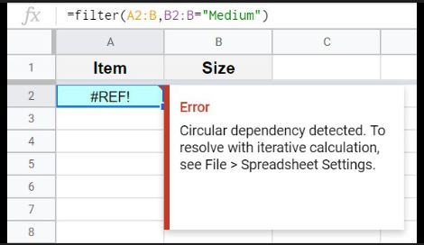
You’re getting a circular dependency error in Google Sheets, and your formula isn’t calculating.
This happens when a formula refers to itself—directly or indirectly—causing Sheets to loop without a result.

This guide shows how to identify and fix it quickly.

Why the Issue Happens

• A formula directly references its own cell
• Two or more cells reference each other (loop)
• Incorrect range includes the formula cell
• Running totals or cumulative formulas built incorrectly
• Copy-paste errors creating hidden circular references
• Misuse of ARRAYFORMULA across overlapping ranges

Step-by-Step Fixes

Step 1: Identify the Circular Reference

Google Sheets usually highlights the cell causing the issue.

Typical example:

= A1 + B1   (entered in A1)

This creates a direct loop.

Fix: Ensure the formula does not reference its own cell.

Step 2: Check for Indirect Loops

Sometimes the loop is not obvious.

Example:

• A1 → refers to B1
• B1 → refers to C1
• C1 → refers back to A1

This creates a circular chain.

Fix: Break the chain by removing one dependency or restructuring formulas.

Step 3: Fix Incorrect Ranges

Very common in totals.

Wrong:

=SUM(A:A)

If this formula is in column A, it includes itself → circular error.

Correct:

=SUM(A1:A99)

Always exclude the formula cell from the range.

Step 4: Fix Running Total Formulas

Incorrect running total:

= B2 + C1   (placed in C2, but copied incorrectly)

This can create loops if structure is wrong.

Correct running total:

= C1 + B2

Ensure:

• First value is fixed
• Each row only refers to previous row, not itself

Step 5: Fix ARRAYFORMULA Overlaps

Problem:

=ARRAYFORMULA(A:A * 2)

If placed in column A → circular dependency.

Fix:

Place in a different column:

=ARRAYFORMULA(A:A * 2)   (placed in column B)

Never apply ARRAYFORMULA on the same column it references.

Step 6: Separate Input and Output Cells

Bad structure:

• Input in A1
• Formula in A1

Fix:

• A1 → input
• B1 → calculation

Example:

B1 = A1 * 10

Keep inputs and formulas separate.

Step 7: Enable Iterative Calculation (Advanced Use Only)

If you intentionally need a circular reference (e.g., interest calculations):

Go to:

• File → Settings → Calculation
• Enable Iterative calculation

Set:

• Max iterations
• Convergence threshold

Use only if you understand the model logic.

Step 8: Trace Dependencies Manually

If you can’t find the error:

• Click the formula cell
• Check all referenced cells
• Follow the chain until you find the loop

Break the loop at any point.

Common Mistakes

• Using SUM(A:A) in column A
• Referencing the same cell inside its own formula
• Copy-pasting formulas without adjusting references
• Using ARRAYFORMULA in the same column
• Creating circular running totals
• Not separating inputs and calculations
• Ignoring indirect circular references

Pro Tips / Better Alternatives

Use Helper Columns

Instead of complex circular formulas, break logic into steps.

Example:

• Column A → raw data
• Column B → intermediate calc
• Column C → final output

This avoids loops and improves clarity.

Use SCAN for Running Totals (Better Method)

Instead of manual running totals:

=SCAN(0, B2:B10, LAMBDA(acc, val, acc + val))

• No circular reference
• Cleaner logic
• Dynamic

Use Absolute References Carefully

Wrong referencing can create loops.

Use $ properly:

= B2 + $C$1

Audit Large Models Regularly

• Check formula dependencies
• Avoid overlapping ranges
• Keep structure modular

Bottom Line

Fix circular dependency errors in this order:

1. Remove self-referencing formulas
2. Check and break indirect loops
3. Fix ranges (exclude formula cell)
4. Separate inputs and outputs
5. Avoid ARRAYFORMULA overlap
6. Use helper columns for complex logic

Circular errors are always structural, not random.
Fix the structure, and the problem disappears.