Google Sheets Conditional Formatting Not Working? Here’s What To Do

Your conditional formatting in Google Sheets isn’t applying correctly, rules don’t trigger, wrong cells are highlighted, or nothing happens at all.
This usually shows up as missing highlights, incorrect matches, or rules that work inconsistently.

This guide fixes it step by step.

Why the Issue Happens

• Wrong range selected for the rule
• Formula references not aligned with the range
• Absolute vs relative reference errors ($)
• Text vs number mismatch
• Extra spaces or hidden characters
• Rule priority conflicts (multiple rules overlapping)
• Incorrect custom formula syntax
• Applying rule to entire column incorrectly

Step-by-Step Fixes

Step 1: Check the Applied Range

Conditional formatting only works within the selected range.

Fix:

• Go to Format → Conditional formatting
• Verify “Apply to range”

Example:

A2:A100

If your data extends beyond this, the rule won’t apply.

Step 2: Use Correct Custom Formula Structure

When using “Custom formula is”, the formula must return TRUE/FALSE.

Correct:

=A2="Sales"

Wrong:

=A2

Always define a condition.

Step 3: Fix Relative vs Absolute References

This is a major source of errors.

Example:

You apply rule to:

A2:C100

Correct formula:

=$B2="Sales"

• $B locks column
• 2 adjusts row dynamically

Wrong:

=B2="Sales"

This shifts incorrectly across columns.

Step 4: Match Data Types (Text vs Number)

If formatting doesn’t trigger, check data type.

Example issue:

• Cell contains "100" (text)
• Rule checks >100 (number)

Fix:

=VALUE(A2)>100

Or ensure column is formatted as number.

Step 5: Remove Extra Spaces

Hidden spaces break matching.

Fix:

=TRIM(A2)="Sales"

If data is messy, clean it first using TRIM.

Step 6: Check Rule Priority

If multiple rules exist, order matters.

Fix:

• Open conditional formatting panel
• Reorder rules (drag up/down)
• Ensure correct rule is on top

Conflicting rules can override each other.

Step 7: Fix Whole Column Rules

If applying to entire column:

A:A

Use:

=A1="Sales"

NOT:

=A2="Sales"

Row reference must match the first row of the range.

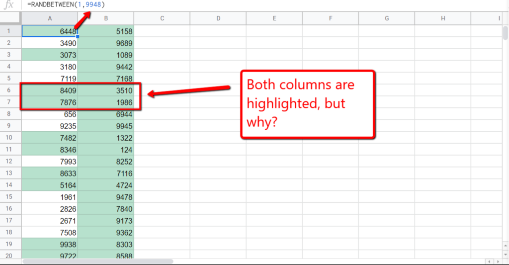
Step 8: Avoid Incorrect Range + Formula Combo

Example issue:

Range:

A2:C100

Formula:

=A2="Sales"

This only checks column A but applies to all columns → inconsistent results.

Fix:

=$A2="Sales"

Step 9: Test with Simple Rule First

If complex rule fails, simplify.

Start with:

=A2="Test"

If this works, gradually add complexity.

Step 10: Reapply Rule (Fix Glitches)

Sometimes formatting bugs occur.

Fix:

• Delete the rule
• Recreate it from scratch

This resolves hidden issues.

Common Mistakes

• Using wrong range
• Incorrect $ usage in formulas
• Ignoring text vs number mismatch
• Not cleaning spaces
• Applying formula to wrong column
• Overlapping rules causing conflicts
• Using incorrect custom formula syntax
• Applying rules to entire column incorrectly

Pro Tips / Better Alternatives

Highlight Entire Rows Based on One Condition

Apply to range:

A2:C100

Formula:

=$B2="Sales"

This highlights full rows based on column B.

Use AND for Multiple Conditions

=AND($B2="Sales", $C2>100)

More precise control.

Use OR for Flexible Conditions

=OR($B2="Sales", $B2="Marketing")

Use ISBLANK to Highlight Missing Data

=ISBLANK(A2)

Use Conditional Formatting for Error Detection

=ISERROR(A2)

Helps identify broken formulas.

Bottom Line

If conditional formatting isn’t working, fix in this order:

1. Verify correct range
2. Fix formula structure (must return TRUE/FALSE)
3. Use proper $ references
4. Match data types
5. Remove extra spaces
6. Check rule priority

Most issues come from reference errors and data inconsistencies.
Fix those, and your conditional formatting will work reliably.