Google Sheets FILTER Function Not Working

Your FILTER function in Google Sheets is returning #N/A, #VALUE!, or empty results when it should return data.
This typically means your conditions don’t match the data, ranges are misaligned, or there’s a data type issue.

This guide fixes it step by step.

Why the Issue Happens

Condition range and data range are different sizes
No matching results (#N/A)
Text vs number mismatch
Extra spaces or hidden characters
Incorrect logical conditions
Using multiple conditions incorrectly
Mixed data types in the same column
Referencing wrong columns

Step-by-Step Fixes

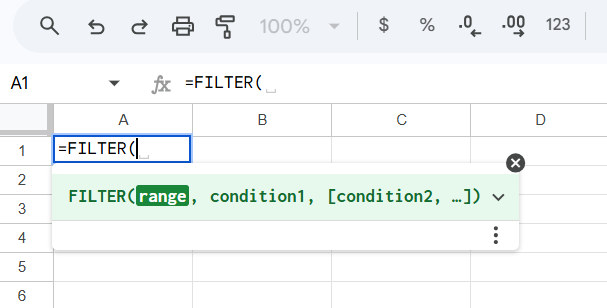
Step 1: Check Basic FILTER Syntax

Correct structure:

=FILTER(range, condition1, [condition2, ...])

Example:

=FILTER(A2:C100, B2:B100="Sales")

range → data to return
condition → must match row-wise

If syntax is wrong, fix this first.

Step 2: Fix Range Size Mismatch

This is a common error (#VALUE!).

Wrong:

=FILTER(A2:C100, B2:B50="Sales")

Ranges must match exactly.

Correct:

=FILTER(A2:C100, B2:B100="Sales")

Step 3: Fix #N/A (No Matches Found)

If no rows meet the condition, FILTER returns #N/A.

Fix with fallback:

=IFERROR(FILTER(A2:C100, B2:B100="Sales"), "No Data")

Also verify:

Does “Sales” actually exist in column B?

Step 4: Fix Text vs Number Mismatch

Example issue:

Column contains "100" (text)
You filter with 100 (number)

Fix:

=FILTER(A2:C100, VALUE(B2:B100)=100)

=FILTER(A2:C100, B2:B100="100")

Match the data type exactly.

Step 5: Remove Extra Spaces

Hidden spaces break matches.

Fix:

=FILTER(A2:C100, TRIM(B2:B100)="Sales")

To clean data:

=ARRAYFORMULA(TRIM(B2:B100))

Step 6: Use Correct Logical Conditions

For numbers:

=FILTER(A2:C100, C2:C100>100)

For text:

=FILTER(A2:C100, B2:B100="Sales")

Avoid mixing conditions incorrectly.

Step 7: Apply Multiple Conditions Correctly

Use * for AND:

=FILTER(A2:C100, (B2:B100="Sales") * (C2:C100>100))

Use + for OR:

=FILTER(A2:C100, (B2:B100="Sales") + (B2:B100="Marketing"))

Incorrect use of commas can break logic.

Step 8: Fix Empty or Blank Conditions

If filtering blanks:

=FILTER(A2:C100, B2:B100<>"")

If blanks exist but are not visible, clean data first.

Step 9: Avoid Full Column References

Using full columns:

=FILTER(A:C, B:B="Sales")

can cause:

Slow performance
Unexpected results

Better:

=FILTER(A2:C1000, B2:B1000="Sales")

Step 10: Debug with Simple Condition

If complex FILTER fails, simplify:

=FILTER(A2:A100, B2:B100="Sales")

Then gradually add conditions.

This isolates the issue.

Common Mistakes

Mismatched range sizes
Expecting results when no match exists
Ignoring text vs number differences
Not removing extra spaces
Using incorrect AND/OR logic
Referencing wrong columns
Using full-column ranges in large datasets

Pro Tips / Better Alternatives

Use QUERY for Complex Filters

=QUERY(A1:C100, "SELECT A, B WHERE C > 100", 1)

Better for structured filtering and large datasets.

Combine FILTER with SORT

=SORT(FILTER(A2:C100, C2:C100>100), 3, FALSE)

Filters and sorts in one step.

Use UNIQUE with FILTER

=UNIQUE(FILTER(A2:A100, B2:B100="Sales"))

Removes duplicates from filtered results.

Use ARRAYFORMULA for Dynamic Data

=ARRAYFORMULA(FILTER(A2:C, B2:B="Sales"))

Expands automatically as data grows.

Clean Data Before Filtering

Use:

=TRIM()
=CLEAN()
=VALUE()

Clean data prevents silent failures.

Bottom Line

If FILTER isn’t working, fix in this order:

Match range sizes exactly
Verify condition actually exists
Fix data types (text vs number)
Remove extra spaces
Apply correct logical conditions
Avoid full column references

Most FILTER issues come from data mismatch and range errors.
Fix those, and your filters will work reliably.